3.3 Discretization

In the following sections we will discretize the contributions to the total energy with the finite element method as shown in Sec. 2. For static energy minimization methods as well as for the calculation of the effective field Eq. (3.14) we have to calculate the derivative of the total energy with respect to the local magnetic polarization $\boldsymbol{J}$. In the following sections we will also derive these gradients.

First we have to define the discrete approximation of the magnetic polarization $\boldsymbol{J}(\boldsymbol{x})$ (Eq. (3.2)) by

$$\boldsymbol{J}(\boldsymbol{x}) \approx J_\mathrm{s}(\bolds... ...,i} \boldsymbol{u}_i \eta_i = \sum_i \boldsymbol{J}_i \quad,$$ (3.10)

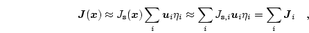
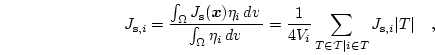
where $\eta_i$ denotes the basis function (hat function) at node $i$ of the finite element mesh. The material parameters $A$, $K$, and $J_\mathrm{s}$ are defined element by element and they are assumed to be constant within each element. However, the magnetic polarization which depends on the saturation polarization $J_\mathrm{s}$ is defined on the nodes. Thus, we have to introduce the node based discrete approximation $J_{\mathrm{s},i}$ of the saturation polarization $J_\mathrm{s}(\boldsymbol{x})$ as

$$J_{\mathrm{s},i}= \frac{ \int_\Omega J_\mathrm{s}(\boldsy... ...\mathcal{T}\vert i \in T} J_{\mathrm{s},i}\vert T\vert \quad,$$ (3.11)

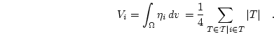
where $V_i$ denotes the volume, which is assigned to node $i$ of the mesh. It is given by

$$V_i= \int_\Omega \eta_i d{v} = \frac{1}{4}\sum_{T \in \mathcal{T}\vert i \in T} \vert T\vert \quad.$$ (3.12)

Since $\boldsymbol{J}$ is a vector with three Cartesian components we have three times the number of nodes unknowns to calculate.

For a given basis $\eta_i$ the total energy can be expanded as

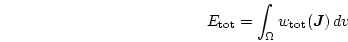$$E_\mathrm{tot}= \int_\Omega w_\mathrm{tot}(\boldsymbol{J}) d{v}$$ (3.13)

and we get for the effective field using the box scheme [40]

$$\boldsymbol{H}_{i,\mathrm{eff}} = -\left( \frac{\delta E_... ...rac{\partial E_\mathrm{tot}}{\partial \boldsymbol{u}_i} \quad.$$ (3.14)