


Next: 3.5 Effective Field
Up: 3. Finite Element Micromagnetics
Previous: 3.3.3 Zeeman Energy
Contents
3.4 Demagnetizing Field and Magnetostatic Energy
The demagnetizing field is a little more complicated to handle, because it is an ``open boundary problem'' with one of its boundary conditions at infinity. In order to overcome this problem Fredkin and Koehler [41,14,42] proposed a hybrid finite element/boundary element method, which requires no finite elements outside the magnetic domain  .
.
Since we assume no free currents in our system, we can calculate the demagnetizing field using a magnetic scalar potential
 . It has to satisfy
with the boundary conditions at the boundary  of
of
 |
(3.36) |
and
 |
(3.37) |
In addition it is required that  for
for
 .
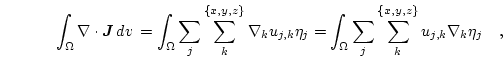
The weak formulation of
.
The weak formulation of
 is simply given by
 |
(3.38) |
which can again be written in matrix-vector format as
 |
(3.39) |
with
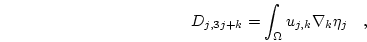 |
(3.40) |
where  stands for the three Cartesian components
  .
.
The main idea now is to split the magnetic scalar potential  into
into  and
and  . Then the problem can be reformulated for these potentials as
 |
(3.41) |
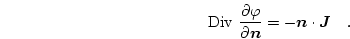
with the boundary condition
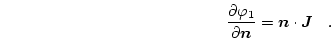 |
(3.42) |
In addition
 for
for
 .
.
As a result, we find for
 |
(3.43) |
with
 |
(3.44) |
and
 |
(3.45) |
It is required that
 for
.
for
.
Potential theory tells us that
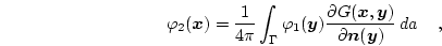 |
(3.46) |
where
 is the Green function.
can be easily calculated using the standard finite element method as explained in Sec. 2.
The (numerically expensive) evaluation of Eq. (3.46) in all can be avoided by just calculating the boundary values of on and then solving the Dirichlet problem Eq. (3.43) with the given boundary values. For
 Eq. (3.46) is given by
 |
(3.47) |
where
 denotes the solid angle subtended by at
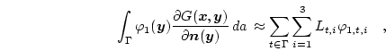
 . Upon triangulation of the surface of the domain with triangular elements (which we naturally get from a triangulation of with tetrahedral elements) and discretization of and we can rewrite Eq. (3.47) as
 |
(3.48) |
with the boundary matrix  , which is a dense matrix with a size of
 elements, where
  is the number of nodes on the surface .
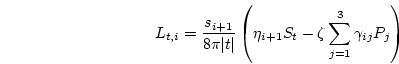
The discretization of the scalar double layer operator in Eq. (3.47) has been derived by Lindholm [43]:
 |
(3.49) |
where  runs over all triangles on the surface of the domain and
  runs over the three nodes of each triangle.
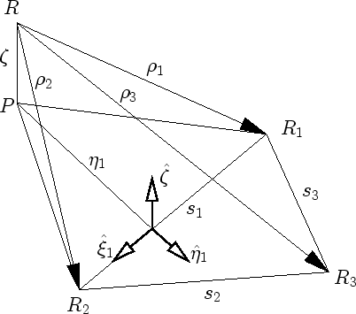
In order to calculate the matrix entries of element by element (rather triangle by triangle) we use the local coordinates defined in Fig. 3.1.
Figure 3.1:
Local coordinate system and various vectors required for the discretization of the boundary integral Eq. (3.47) [43].
 |
 |
(3.50) |
 |
 |
 |
(3.51) |
 |
|
 |
(3.52) |
 |
|
 |
(3.53) |
 |
|
 |
(3.54) |
 |
|
 |
(3.55) |
 |
|
 |
(3.56) |
 denotes the area of triangle and
  the solid angle subtended by triangle at the ``observation point''
 ,
which is given by
,
which is given by
 |
(3.57) |
In order to calculate the demagnetizing field, we have to perform the following steps:
Initialization
- Discretize Eq. (3.41).
- Calculate the boundary matrix in Eq. (3.48).
Solution
- Solve Eq. (3.41) for a given magnetization distribution
 using the standard FE method.
- Calculate on the boundary using Eq. (3.48) to get the values for the Dirichlet boundary conditions.
- Calculate in the whole domain using Eq. (3.43) with Dirichlet boundary values.
- Calculate
 .
.
Next: 3.5 Effective Field
Up: 3. Finite Element Micromagnetics
Previous: 3.3.3 Zeeman Energy
Contents
Werner Scholz
2003-06-08