2.3 Galerkin Discretization

In order to solve the Poisson problem numerically we have to discretize the weak formulation of the Poisson equation (Eq. (2.8)) and restrict the solution space of the numerical solution $U$ to a finite dimensional subspace $S$ of $H^1(\Omega)$. Accordingly $U_D \in S_D := S \cap H^1_D$ approximates $u_D$ on $\Gamma_D$. The discretized problem $P_S$ can then be written as: Find $V \in S_D$ such that

$$\int_\Omega \nabla V \cdot \nabla W d{v} = \int_\Omega... ...t W d{a} - \int_\Omega \nabla U_D \cdot \nabla W d{v}$$ (2.9)

with $W \in S_D$.

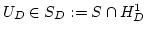
If we assume that $(\eta_1, \ldots, \eta_N)$ is a basis of the $N$-dimensional space 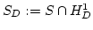$S$ and $S_D := S \cap H^1_D$ a $M$-dimensional subspace then we can rewrite Eq. (2.9)

$$\int_\Omega \nabla V \cdot \nabla \eta_j d{v} = \int_\... ...nabla U_D \cdot \nabla \eta_j d{v} (\eta_j \in S_D) \quad.$$ (2.10)

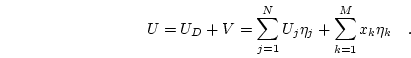
If we now make a series expansion of $V$ and $U_D$ in terms of $\eta_k$

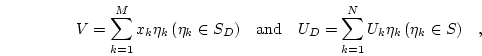$$V=\sum_{k=1}^{M} x_k \eta_k (\eta_k \in S_D) \quad\mathr... ...}\quad U_D=\sum_{k=1}^{N} U_k \eta_k (\eta_k \in S) \quad,$$ (2.11)

then we obtain

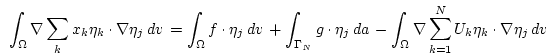$$\int_\Omega \nabla \sum_k x_k \eta_k \cdot \nabla \eta_j ... ... \nabla \sum_{k=1}^{N} U_k \eta_k \cdot \nabla \eta_j d{v}$$ (2.12)

which can be rewritten as

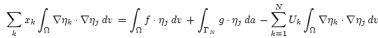$$\sum_k x_k \int_\Omega \nabla \eta_k \cdot \nabla \eta_j ... ...{N} U_k \int_\Omega \nabla \eta_k \cdot \nabla \eta_j d{v}$$ (2.13)

and finally simplified to a system of linear equations

$$A x = b$$ (2.14)

where the ``stiffness matrix'' is given by

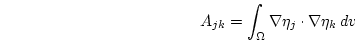$$A_{jk} = \int_\Omega \nabla \eta_j \cdot \nabla \eta_k d{v}$$ (2.15)

and the ``right hand side'' by

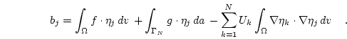$$b_j = \int_\Omega f \cdot \eta_j d{v} + \int_{\Gamma... ... \int_\Omega \nabla \eta_k \cdot \nabla \eta_j d{v} \quad.$$ (2.16)

The stiffness matrix is sparse, symmetric, and positive definite. Thus, Eq. (2.14) has exactly one solution $x \in \mathbb{R}^M$, which gives the Galerkin solution

$$U=U_D+V=\sum_{j=1}^{N} U_j \eta_j + \sum_{k=1}^{M} x_k \eta_k \quad.$$ (2.17)